1 Overview of Methods

(1) Drought analysis: two meteorological drought indices, i.e., Standardized Precipitation Evapotranspiration Index (SPEI) and Standardized Precipitation Index (SPI), were adopted to investigate the drought characteristics in the LMRB. Two sets of long-term reanalysis dataset, i.e., Climate Research Unit gridded Time Series (CRU TS) dataset from 1901 to 2019 and Climate Hazards Group Infrared Precipitation with Station data (CHIRPS) dataset from 1981 to 2019, were adopted for analysis.

(2) Runoff composition analysis: a distributed hydrological model (THREW) was established for the whole LMRB. The model was calibrated and verified against the observed discharge at 8 main hydrological stations along the mainstream of Lancang-Mekong River (as listed in Table 1). We chose the period of 1991-2001 to calibrate and validate the model when large dams have not been commissioned yet and a sufficient number of rain gauges are available. The parameters and construction years of major commissioned dams on the Lancang River are detailed in Table 2. According to data retrieved from MRC, the number of available rain gauges (see Figure 2 for details) became much less after 2005, so we also used satellite rainfall products (GPM IMERG) to drive the model, which is available from 2001-2019. We chose the overlap period of 2001-2005 to validate the accuracy of GPM driven simulations. The runoff compositions at 8 hydrological stations were then investigated based on the modelling results. 

(3) Impacts of reservoir regulation on streamflow along the Mekong River: the natural runoff at the Chiang Saen Hydrological Station in Thailand was reconstructed by using the distributed hydrological model THREW from 1991-2019 driven by integrated rainfall time series data (rain gauge measurements and satellite rainfall product). The impacts of reservoir regulation on streamflow was then investigated by comparing the reconstructed natural flow and observed flow at Chiang Saen Hydrological Station during different time periods. According to the construction years of major dams (in Table 2), we chose the period of 1991-2001 as a quasi-natural period without significant dam perturbation. During this period, only Manwan reservoir was commissioned in 1995 with total storage of 887 MCM (million cubic meter), which can be ignorable compared to the annual mean discharge of 56200 MCM at Jinghong (MRC and MWR of China, 2016). We then chose the period of 2010-2019 as an altered period as two major dams (Xiaowan Dam and Nuozhadu Dam) were commissioned in 2010 and 2014, respectively. Table 2. Parameters and construction years of major dams on the Lancang River (WLE, 2018)

Project name	Commercial Operation Date	Dead storage  (MCM)	Total storage  (MCM)
Manwan	1992	630	887
Dachaoshan	2003	465	740
Jinghong	2009	810	1119
Xiaowan	2010	4750	14645
Gongguoqiao	2012	196	316
Nuozhadu	2014	10414	21749
Miaowei	2016	359	660
Huangdeng	2017	1031	1418
Wunonglong	2018	236	272
Dahuaqiao	2018	252	293
Lidi	2019	57	71

  

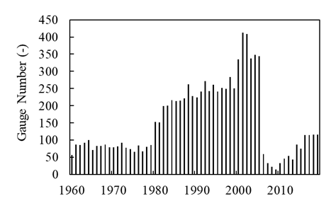
Figure 2. Number of available rain gauges from 1960 to 2019 in the Mekong River Basin 

2 Hydrological and meteorological data 

(1) Gauged rainfall and meteorological data were obtained from MRC and the China Meteorological Administration (CMA). For the Mekong sub-region, we collected daily data from 166 rain gauges and 32 meteorological gauges from 1991 to 2005 with high-quality temporal continuity. For the Lancang sub-region, we collected data from 12 rain gauges and 12 meteorological gauges with the continuous record during the same period. Meteorological data contain near-surface air pressure, air temperature, air specific humidity, wind speed and direction, sunshine duration, and solar radiation. They were used to calculate potential evapotranspiration based on the Penman-Monteith Equation, which is an important input for the THREW model. 

(2) The gauged daily runoff data in 1991-2019 were collected from MRC and MWR of China for the main hydrological stations along the Lancang-Mekong River (i.e., Jinghong, Chiang Saen, Luang Prabang, Nong Khai, Nakhon Phanom, Mukdahan, Pakse, and Stung Treng).  

(3) As the number of available rain gauges became significantly less after 2005, the IMERG Final Run dataset was adopted for the hydrological simulation during the recent 14 years from 2006 to 2019. IMERG is a satellite rainfall product released by GPM (Global Precipitation Measurement) project. A number of studies show that the IMERG product performs quite well in Southeast Asia (Li et al., 2019; Wang et al., 2017; He et al., 2017).  

(4) The CRU TS (Climate Research Unit gridded Time Series) global reanalysis meteorological dataset and the CHIRPS (Climate Hazards Group Infrared Precipitation with Station data) precipitation dataset were chosen for the drought analysis. CRU TS is one of the most widely used observed climate datasets and is produced by the UK’s National Centre for Atmospheric Science (NCAS) at the University of East Anglia’s Climatic Research Unit (CRU). CRU TS provides monthly data on a 0.5° x 0.5° grid covering global land surfaces (except Antarctica) from 1901 to 2019. There are ten variables, all based on near-surface measurements: temperature (mean, minimum, maximum and diurnal range), precipitation (total, also rain day counts), humidity (as vapour pressure), frost day counts, cloud cover, and potential evapotranspiration. It has been widely used in meteorological and hydrological studies (Harris et al., 2020). Based on the CRU TS dataset, this study extracted the precipitation and potential evapotranspiration data of the LMRB in the past 119 years (1901-2019). CHIRPS precipitation dataset is jointly developed by the United States Geological Survey (USGS) and the University of California, Santa Barbara, with a sequence length of 1981 to the near present and a finer spatial resolution of 0.05°×0.05°. CHIRPS precipitation data has been successfully applied to meteorological drought analysis in the Lower Mekong Basin (Guo et al., 2017). The monthly precipitation data of CHIRPS from 1981-2019 was used in this study with the purpose of comparison with CRU TS. 

3 Drought analysis method 

(1) Meteorological drought index 

In this study, two meteorological indices, the Standardized Precipitation Evapotranspiration Index (SPEI) and the Standardized Precipitation Index (SPI), were adopted for drought analysis.  

The standardized precipitation index (SPI), for measuring the excess and deficit of precipitation on various temporal scales, is a widely adopted metric for drought diagnosis. The typical procedure to calculate SPI is as follows: 1) Γ distribution probability is adopted to describe precipitation in the SPI calculation; 2) Normal standardization of skewed probability distribution is conducted; 3) Drought is graded using the distribution of cumulative frequency of standardized precipitation. The SPI is an indicator expressing the precipitation occurrence probability in a given period that is applicable to meteorological drought monitoring and evaluation on or above the monthly scale. With the advantages of easy access to data, easy calculation, flexible temporal scale, and regional comparability, SPI has been widely applied to the depiction of meteorological drought in recent years. The formulae to calculate SPI are as follows (McKee et al., 1993):  

 

 

In specific, x is precipitation sample value; S is the positive and negative coefficients of probability density; c0, c1, c2 and d1, d2, d3 are calculation parameters of the simplified approximation analysis formula for converting Γ distribution probability into cumulative frequency, and c0=2.515517, c1=0.802853, c2=0.010328, d1=1.432788, d2=0.189269 and d3=0.001308. G(x) is the rainfall distribution probability related to Γ function. According to the probability density integral formula of Γ function is:  

 

  

 

where, S = 1 when G(x) > 0.5, S = -1 when G(x) ≤ 0.5.  

The procedure for calculating the SPEI is similar to that for the SPI. However, the SPEI uses the “climatic water balance” concept, the difference between precipitation and potential evapotranspiration (P-ET0), rather than precipitation (P) as the input (Beguería et al., 2014).  

The time scale for SPI / SPEI calculation can range from 1 to 48 months or longer, expressed as SPEI 1… SPEI48（SPI1… SPI48), etc. The small scale SPEI / SPI index is used to represent the short-term drought while the longer scale index, such as SPEI12 / SPI12, reflects the inter-annual fluctuation. If the consecutive 12-month period is not significantly wet or dry, the index will be close to 0 (WMO, 2012). Considering the influence of long-term drought is more significant, the 12-month scale index (SPI12 and SPEI12) is used in the analysis of long-term drought characteristics. The 3-month index is used to analyse the characteristics of drought in a short time scale. In particular, we adopted SPEI3 and SPI3 to investigate the course of a typical drought event occurred in 2019. 

Taking into consideration of the influence of evaporation on drought severity, SPEI can better reflect the impacts of drought on the hydrological system and ecosystem than SPI based on precipitation only. Therefore, this study principally adopted SPEI index to investigate the drought characteristics, which is calculated based on precipitation and potential evapotranspiration data of CRU TS from 1901-2019. At the same time, we also calculated the SPI index based on the CHIRPS data from 1981-2019 as an independent validation. 

The drought grades of SPEI / SPI are evaluated according to the Chinese National Standard <Grades of Meteorological Drought> (GB / T 20481-2017) and the WMO User Guide. The detail is shown in Table 3. It indicates that the two grading systems have the same thresholds for moderate, severe, and exceptional droughts. 

Table 3. Grades of SPEI/SPI 

Grade	Type		SPEI/SPI
China		China / WMO	WMO	China
I		No drought	>0.0	>-0.5
II		Mild drought	(-1.0, 0.0)	(-1.0, -0.5)
III		Moderate drought	(-1.5, -1.0)	(-1.5, -1.0)
IV		Severe drought	(-2.0, -1.5)	(-2.0, -1.5)
V		Exceptional drought	≤-2.0	≤-2.0

(2) Frequency of drought 
In this study, we principally investigated the frequency characteristics of drought. The frequency of drought refers to the number of occurrences of drought in the entire period of time. The calculation formula is: 

d = (n/N) × 100%   (4) 

where, n is the number of months drought occurs, N is the entire sequence length. 

4 Distributed hydrological model  

We adopted the THREW model (Tsinghua Hydrological Model based on Representative Elementary Watershed) to simulate the natural runoff in the LMRB. This model was developed by Fuqiang Tian in Tsinghua University on the basis of the Representative Elementary Watershed method proposed by Murugesu Sivapalan in the University of Illinois Urbana Champaign. The important processes including glacier and snow melting were incorporated into the model to make it applicable to cold regions. The model has been successfully applied in several watersheds with different climate and landscape configurations, e.g., Illinois River Basin in the USA (Li et al., 2012; Tian et al., 2012), Lientz Basin in Austria (He et al., 2014), Hanjiang River Basin (Sun et al., 2014) and Urumqi River Basin in China (Mou et al., 2009), and Yarlung Zangbo-Brahmaputra River Basin (Xu et al., 2019). 

The LMRB was divided into 595 sub-basins based on the 1×1km2 resolution Digital Elevation Model (DEM) using the Pfafstetter method. The 33 sub-basins whose area is larger than 5000 km2 were divided into smaller ones and the whole study area was finally divided into 651 representative elementary watersheds (REWs). Each of the REW was further divided into seven sub-zones, i.e., snow-covered zone (n-zone), saturated zone (s-zone), unsaturated zone (u-zone), vegetable covered zone (v-zone), bared zone (b-zone), sub-stream network zone (t-zone) and main channel reach zone (r-zone). 

The soil hydraulic parameters were derived from the soil classification data which are extracted from the 10 km global digital soil map provided by the Food and Agriculture Organization of the United Nations (FAO). For the Leaf Area Index (LAI) data, the Normalized Difference Vegetation Index (NDVI) data, and the snow cover data, the MODIS data are used, with a spatial resolution of 500×500m, and temporal resolution of 16 days. 

The daily runoff data during 1991-2001 at 8 hydrological stations along the Lancang-Mekong mainstream are used to calibrate and validate the model in a spatially distributed way. The calibration method is detailed as follows: 1) The discharge during the wet season (from June to November) and dry season (from December to May) are calibrated separately, and the simulated discharge of the two periods are then combined together; 2) The discharge at 8 stations is calibrated from upstream to downstream; 3) Once the calibration is finished at an upstream station, the parameters for the REWs draining to this station are fixed, and the discharge of the next downstream station is used to calibrate the parameters for the REWs located in the inter-region between the two stations. The whole period of 1991 to 2001 was divided into two sub-periods, which were used for model calibration (1991-1996) and validation (1997-2001) respectively. The simulation time step is daily, and the widely used model evaluation metrics (NSE, lnNSE, and RE) are chosen as objective functions to calibrate and validate the model, which are calculated by the following equations: 

 

 

Figure 3 shows the simulated and observed daily streamflow at 8 stations, and Table 4 shows the values of evaluation metrics. The NSE and lnNSE at Jinghong station during the verification period are between 0.85 and 0.9, those of the other stations are around or larger than 0.9, and RE are all lower than ±5%. In general, the THREW model performs quite well in simulating the streamflow in the LMRB.  

 

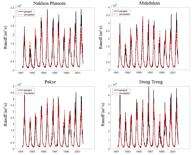
Figure 3. Simulated and observed daily streamflow at the 8 stations along the mainstream of the Lancang-Mekong River

Table 4. Evaluation metrics of THREW model simulation in the LMRB 

Hydrological Gauge	Driven by gauge rainfall data					Driven by IMERG rainfall data
	Calibration		Validation		RE	(2001-2005) NSE
	(1991-1996)		(1997-2001)
	NSE	lnNSE	NSE	lnNSE
Jinghong	0.86	0.78	0.89	0.85	-3.22%	0.89
Chiang Saen	0.88	0.85	0.9	0.92	1.31%	0.95
Luang Prabang	0.88	0.89	0.92	0.94	3.21%	0.94
Nong Khai	0.92	0.93	0.92	0.95	3.23%	0.95
Nakhon Phanom	0.92	0.92	0.89	0.94	-3.57%	0.9
Mukdahan	0.94	0.93	0.93	0.95	4.92%	0.89
Pakse	0.94	0.95	0.91	0.95	0.72%	0.87
Stung Treng	0.92	0.92	0.89	0.93	2.60%	0.87
Average	0.91	0.9	0.91	0.93	-	0.91

2.5 Runoff simulation driven by IMERG rainfall product 

Figure 4 shows the streamflow simulation results in 2001-2005 driven by gauge rainfall data and satellite rainfall data respectively. The last column of Table 4 shows the NSE calculated by the IMERG rainfall driven streamflow and gauge rainfall driven streamflow. The results indicate high accuracy of the THREW model (NSE > 0.85) driven by IMERG rainfall product. The reason we used gauge rainfall based simulation results as the reference value is that there was another dam commissioned in 2003, which could alter the streamflow to some extent (see Table 2).  

 

 

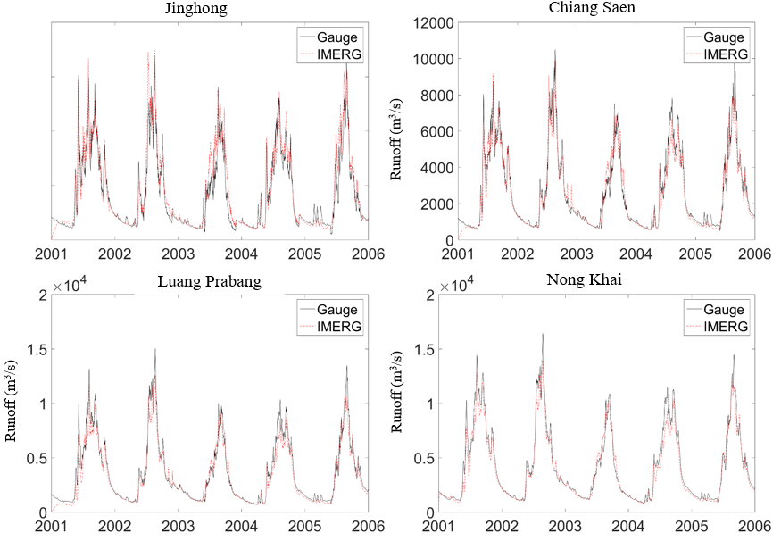
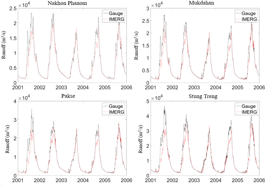
Figure 4. Streamflow simulation driven by the satellite rainfall and the gauge rainfall at 8 hydrological stations along the mainstream of Lancang-Mekong River